Problems for Chapter 3
Problem III-1. Use an argument like the one given in the text for the Coulomb force to show that $\int_C \mathbf{F} \cdot \hat{\mathbf{t}} \\, ds = 0$ is independent of path for any central force $\mathbf{F}$.
Solution. Click to Expand
If $\mathbf{F}$ is a central force, then for any point $P$ in space, the force is in the radial direction and its magnitude depends only on the distance $r$ from the origin:
$$ \mathbf{F} = F_r(r) \hat{\mathbf{e}}_r $$
Then we have:
$$ \begin{align*} F_x &= F_r(r) \sin \phi \cos \theta \\ F_y &= F_r(r) \sin \phi \sin \theta \\ F_z &= F_r(r) \cos \phi \end{align*} $$
and since:
$$ \begin{align*} x &= r \sin \phi \cos \theta \\ y &= r \sin \phi \sin \theta \\ z &= r \cos \phi \end{align*} $$
We have:
$$ \begin{align*} dx &= \sin \phi \cos \theta \, dr + r \cos \phi \cos \theta \, d\phi - r \sin \phi \sin \theta \, d\theta \\ dy &= \sin \phi \sin \theta \, dr + r \cos \phi \sin \theta \, d\phi + r \sin \phi \cos \theta \, d\theta \\ dz &= \cos \phi \, dr - r \sin \phi \, d\phi \end{align*} $$
Then:
$$ \begin{align*} F_x \, dx &+ F_y \, dy + F_z \, dz = \\ & F_r(r) (\sin^2 \phi \cos^2 \theta + \sin^2 \phi \sin^2 \theta + \cos^2 \phi) \, dr + \\ & F_r(r) (r \sin \phi \cos \phi \cos^2 \theta + r \sin \phi \cos \phi \sin^2 \theta - r \sin \phi \cos \phi) \, d\phi + \\ & F_r(r) (-r \sin^2 \phi \sin \theta \cos \theta + r \sin^2 \phi \sin \theta \cos \theta) \, d\theta \end{align*} $$
Which simplifies to:
$$ F_x \, dx + F_y \, dy + F_z \, dz = F_r(r) \, dr $$
On page 68 we saw that:
$$ \int_C \mathbf{F} \cdot \hat{\mathbf{t}} \, ds = \int_C (F_x \, dx + F_y \, dy + F_z \, dz) $$
Thus, we have:
$$ \begin{align*} \int_C \mathbf{F} \cdot \hat{\mathbf{t}} \, ds &= \int_C F_r(r) \, dr \\ &= \int_{r_1}^{r_2} F_r(r) \, dr \end{align*} $$
which is independent of the path taken and depends only on the initial and final radius.
Problem III-2. In the text we obtained the result
$$ (\nabla \times \mathbf{F})_z = \frac{\partial F_y}{\partial x} - \frac{\partial F_x}{\partial y} $$
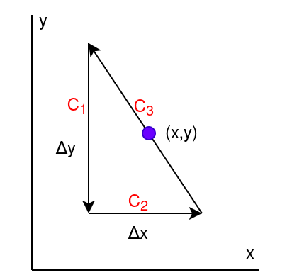
by integrating over a small rectanglular path. As an example of the fact that this result is independent of the path, rederive it, using a triangular path.
Solution. Click to Expand
Assume the force $\mathbf{F}$ is given by:
$$ \mathbf{F} = F_x \mathbf{i} + F_y \mathbf{j} + F_z \mathbf{k} $$
In the text on page 68 we saw that:
$$ \int_C \mathbf{F} \cdot \hat{\mathbf{t}} \, ds = \int_C (F_x \, dx + F_y \, dy + F_z \, dz) $$
Then for $C_1$, we have:
$$ \begin{align*} \int_{C_1} \mathbf{F} \cdot \hat{\mathbf{t}} \, ds &= \int_{y + \Delta y / 2}^{y - \Delta y / 2} F_y\left(x - \frac{\Delta x}{2} , u\right) \, du \\[1em] & \approx -F_y\left(x - \frac{\Delta x}{2} , y\right) \Delta y \end{align*} $$
and for $C_2$, we have:
$$ \begin{align*} \int_{C_2} \mathbf{F} \cdot \hat{\mathbf{t}} \, ds &= \int_{x - \Delta x / 2}^{x + \Delta x / 2} F_x\left(u, y - \frac{\Delta y}{2}\right) \, du \\[1em] & \approx F_x\left(x, y - \frac{\Delta y}{2}\right) \Delta x \end{align*} $$
and for $C_3$, we have:
$$ \begin{align*} \int_{C_3} \mathbf{F} \cdot \hat{\mathbf{t}} \, ds &= \int_{C_3} \left( F_x \, dx + F_y \, dy \right) \\[1em] &= \int_{x + \Delta x / 2}^{x - \Delta x / 2} F_x\left(u, y(u)\right) \, du + \int_{y - \Delta y / 2}^{y + \Delta y / 2} F_y\left(x(u), u\right) \, du \\[1em] & \approx -F_x\left(x, y\right) \Delta x + F_y\left(x, y\right) \Delta y \end{align*} $$
Thus, we have:
$$ \begin{align*} \int_{C_1+C_2+C_3} \mathbf{F} &\cdot \hat{\mathbf{t}} \, ds \approx \\[0.5em] &\Delta y \left( F_y(x, y) - F_y\left(x - \frac{\Delta x}{2}, y\right) \right) + \\[0.5em] &\Delta x \left( F_x\left(x, y - \frac{\Delta y}{2}\right) - F_x(x, y) \right) \end{align*} $$
Since $\Delta A = \dfrac{\Delta x \Delta y}{2}$, we have:
$$ \begin{align*} \frac{1}{\Delta A} \int_{C_1+C_2+C_3} \mathbf{F} &\cdot \hat{\mathbf{t}} \, ds \approx \\[0.5em] & \frac{F_y(x, y) - F_y\left(x - \frac{\Delta x}{2}, y\right)} {\Delta x / 2} - \\[0.5em] &\frac{F_x(x, y) - F_x\left(x, y - \frac{\Delta y}{2}\right)}{\Delta y / 2} \end{align*} $$
So, we have:
$$ \lim_{\Delta A \to 0} \frac{1}{\Delta A} \int_{C_1+C_2+C_3} \mathbf{F} \cdot \hat{\mathbf{t}} \, ds = \frac{\partial F_y}{\partial x} - \frac{\partial F_x}{\partial y} $$
Problem III-7. Show that $\nabla \cdot (\nabla \times \mathbf{F}) = 0$. (Assume that mixed second partial derivatives are independent of the order of differentiation.)
Solution. Click to Expand
$$ \begin{align*} \nabla \times \mathbf{F} &= \mathbf{i} \left( \frac{\partial F_z}{\partial y} - \frac{\partial F_y}{\partial z} \right) \\ &+ \mathbf{j} \left( \frac{\partial F_x}{\partial z} - \frac{\partial F_z}{\partial x} \right) \\ &+ \mathbf{k} \left( \frac{\partial F_y}{\partial x} - \frac{\partial F_x}{\partial y} \right) \end{align*} $$
Then:
$$ \begin{align*} \nabla \cdot (\nabla \times \mathbf{F}) &= \frac{\partial F_z}{\partial x \partial y} - \frac{\partial F_y}{\partial x \partial z} \\ &+ \frac{\partial F_x}{\partial y \partial z} - \frac{\partial F_z}{\partial x \partial y} \\ &+ \frac{\partial F_y}{\partial x \partial z} - \frac{\partial F_x}{\partial y \partial z} \\ &= 0 \end{align*} $$
Problem III-8. In the text we obtained the $z$-component of $\nabla \times \mathbf{F}$ in cylindrical coordinates. Proceeding the same way, obtain the $\theta$- and $r$-components.
Solution ($\theta$-component). Click to Expand
Using the path shown in the figure, we’ll yield the $\theta$-component of $\nabla \times \mathbf{F}$ in cylindrical coordinates.
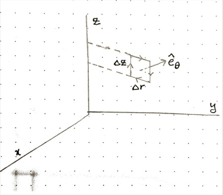
Viewed from above:
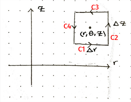
For $C_1$, we have $\hat{\mathbf{t}} = \hat{\mathbf{e}_r}$ and $ds = dr$. Then:
$$ \begin{align*} \int_{C_1} \mathbf{F} \cdot \hat{\mathbf{t}} \, ds &= \int_{r - \Delta r / 2}^{r + \Delta r / 2} F_r(u, \theta, z - \frac{\Delta z}{2}) \, du \\[1em] &\approx F_r(r, \theta, z - \frac{\Delta z}{2}) \Delta r \end{align*} $$
For $C_2$, we have $\hat{\mathbf{t}} = \mathbf{\mathbf{e}_z}$ and $ds = dz$. Then:
$$ \begin{align*} \int_{C_2} \mathbf{F} \cdot \hat{\mathbf{t}} \, ds &= \int_{z - \Delta z / 2}^{z + \Delta z / 2} F_z(r + \Delta r / 2, \theta, u) \, du \\[1em] &\approx F_z(r + \frac{\Delta r}{2}, \theta, z) \Delta z \end{align*} $$
For $C_3$, we have $\hat{\mathbf{t}} = -\hat{\mathbf{e}_r}$ and $ds = -dr$. Then:
$$ \begin{align*} \int_{C_3} \mathbf{F} \cdot \hat{\mathbf{t}} \, ds &= \int_{r + \Delta r / 2}^{r - \Delta r / 2} (-F_r(u, \theta, z + \frac{\Delta z}{2})) \, (-du) \\[1em] &\approx -F_r(r, \theta, z + \frac{\Delta z}{2}) \Delta r \end{align*} $$
For $C_4$, we have $\hat{\mathbf{t}} = -\hat{\mathbf{e}_z}$ and $ds = -dz$. Then:
$$ \begin{align*} \int_{C_4} \mathbf{F} \cdot \hat{\mathbf{t}} \, ds &= \int_{z + \Delta z / 2}^{z - \Delta z / 2} (-F_z(r - \Delta r / 2, \theta, u)) \, (-du) \\[1em] &\approx -F_z(r - \frac{\Delta r}{2}, \theta, z) \Delta z \end{align*} $$
Then, we have:
$$ \begin{align*} \int_{C_1 + C_2 + C_3 + C_4} \mathbf{F} &\cdot \hat{\mathbf{t}} \, ds \approx \\[0.5em] &\Delta r \left( F_r(r, \theta, z - \frac{\Delta z}{2}) - F_r(r, \theta, z + \frac{\Delta z}{2}) \right) + \\[0.5em] &\Delta z \left( F_z(r + \frac{\Delta r}{2}, \theta, z) - F_z(r - \frac{\Delta r}{2}, \theta, z) \right) \end{align*} $$
Since $\Delta A = \Delta r \Delta z$, we have:
$$ \begin{align*} \frac{1}{\Delta A} \int_{C_1 + C_2 + C_3 + C_4} \mathbf{F} &\cdot \hat{\mathbf{t}} \, ds \approx \\[0.5em] & \frac{F_r(r, \theta, z - \dfrac{\Delta z}{2}) - F_r(r, \theta, z + \dfrac{\Delta z}{2})} {\Delta z} - \\[0.5em] &\frac{F_z(r + \dfrac{\Delta r}{2}, \theta, z) - F_z(r - \dfrac{\Delta r}{2}, \theta, z)}{\Delta r} \end{align*} $$
So, $\theta$-component of $\nabla \times \mathbf{F}$ is:
$$ \lim_{\Delta A \to 0} \frac{1}{\Delta A} \int_{C_1 + C_2 + C_3 + C_4} \mathbf{F} \cdot \hat{\mathbf{t}} \, ds = \frac{\partial F_r}{\partial z} - \frac{\partial F_z}{\partial r} $$
Solution ($r$-component). Click to Expand
Using the path shown in the figure, we’ll yield the $r$-component of $\nabla \times \mathbf{F}$ in cylindrical coordinates.
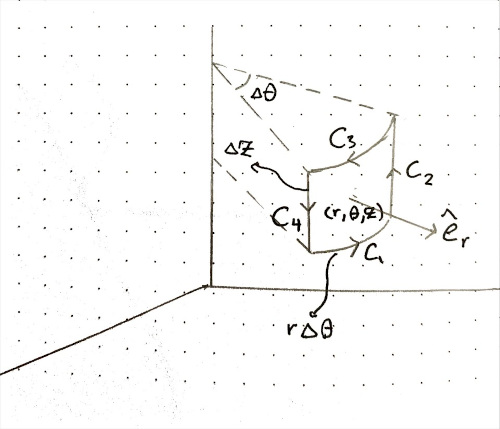
For $C_1$, we have $\hat{\mathbf{t}} = \hat{\mathbf{e}_\theta}$ and $ds = r d\theta$. Then:
$$ \begin{align*} \int_{C_1} \mathbf{F} \cdot \hat{\mathbf{t}} \, ds &= \int_{\theta - \Delta \theta / 2}^{\theta + \Delta \theta / 2} F_\theta(r, u, z - \frac{\Delta z}{2}) \, r \, du \\[1em] &\approx F_\theta(r, \theta, z - \frac{\Delta z}{2}) r \Delta \theta \end{align*} $$
For $C_2$, we have $\hat{\mathbf{t}} = \hat{\mathbf{e}_z}$ and $ds = dz$. Then:
$$ \begin{align*} \int_{C_2} \mathbf{F} \cdot \hat{\mathbf{t}} \, ds &= \int_{z - \Delta z / 2}^{z + \Delta z / 2} F_z(r, \theta + \frac{\Delta \theta}{2}, u) \, du \\[1em] &\approx F_z(r, \theta + \frac{\Delta \theta}{2}, z) \Delta z \end{align*} $$
For $C_3$, we have $\hat{\mathbf{t}} = -\hat{\mathbf{e}_\theta}$ and $ds = -r d\theta$. Then:
$$ \begin{align*} \int_{C_3} \mathbf{F} \cdot \hat{\mathbf{t}} \, ds &= \int_{\theta + \Delta \theta / 2}^{\theta - \Delta \theta / 2} (-F_\theta(r, u, z + \frac{\Delta z}{2})) \, (-r \, du) \\[1em] &\approx -F_\theta(r, \theta, z + \frac{\Delta z}{2}) r \Delta \theta \end{align*} $$
For $C_4$, we have $\hat{\mathbf{t}} = -\hat{\mathbf{e}_z}$ and $ds = -dz$. Then:
$$ \begin{align*} \int_{C_4} \mathbf{F} \cdot \hat{\mathbf{t}} \, ds &= \int_{z + \Delta z / 2}^{z - \Delta z / 2} (-F_z(r, \theta - \frac{\Delta \theta}{2}, u)) \, (-du) \\[1em] &\approx -F_z(r, \theta - \frac{\Delta \theta}{2}, z) \Delta z \end{align*} $$
Then, we have:
$$ \begin{align*} \int_{C_1 + C_2 + C_3 + C_4} \mathbf{F} &\cdot \hat{\mathbf{t}} \, ds \approx \\[0.5em] &r \, \Delta \theta \left( F_\theta(r, \theta, z - \frac{\Delta z}{2}) - F_\theta(r, \theta, z + \frac{\Delta z}{2}) \right) + \\[0.5em] &\Delta z \left( F_z(r, \theta + \frac{\Delta \theta}{2}, z) - F_z(r, \theta - \frac{\Delta \theta}{2}, z) \right) \end{align*} $$
Since $\Delta A = r \Delta \theta \Delta z$, we have:
$$ \begin{align*} \frac{1}{\Delta A} \int_{C_1 + C_2 + C_3 + C_4} \mathbf{F} &\cdot \hat{\mathbf{t}} \, ds \approx \\[0.5em] & \frac{F_z(r, \theta + \dfrac{\Delta \theta}{2}, z) - F_z(r, \theta - \dfrac{\Delta \theta}{2}, z)} {r \, \Delta \theta} - \\[0.5em] &\frac{F_\theta(r, \theta, z + \dfrac{\Delta z}{2}) - F_\theta(r, \theta, z - \dfrac{\Delta z}{2})}{\Delta z} \end{align*} $$
So, $r$-component of $\nabla \times \mathbf{F}$ is:
$$ \lim_{\Delta A \to 0} \frac{1}{\Delta A} \int_{C_1 + C_2 + C_3 + C_4} \mathbf{F} \cdot \hat{\mathbf{t}} \, ds = \frac{1}{r} \, \frac{\partial F_z}{\partial \theta} - \frac{\partial F_{\theta}}{\partial z} $$
Problem III-14. Use Stokes’ theorem to show that
$$ \oint_C \hat{\mathbf{t}} \, ds = 0 $$
Solution. Click to Expand
Using $\nabla \times \mathbf{F} = \mathbf{i} \left( \frac{\partial{F_z}}{\partial y} - \frac{\partial{F_y}}{\partial z} \right) + \mathbf{j} \left( \frac{\partial{F_x}}{\partial z} - \frac{\partial{F_z}}{\partial x} \right) + \mathbf{k} \left( \frac{\partial{F_y}}{\partial x} - \frac{\partial{F_x}}{\partial y} \right)$, we get: $\nabla \times \mathbf{i}$ = $\nabla \times \mathbf{j}$ = $\nabla \times \mathbf{k} = 0$.
Then, $i$-component of $\oint_C \hat{\mathbf{t}} \\, ds$ is:
$$ \begin{align*} \mathbf{i} \cdot \oint_C \hat{\mathbf{t}} \, ds &= \oint_C \mathbf{i} \cdot \hat{\mathbf{t}} \, ds \\ &= \iint_S \nabla \times \mathbf{i} \cdot \hat{\mathbf{n}} \, dS \\ &= 0 \end{align*} $$
Similarly, we can show that $j$-component and $k$-component of $\oint_C \hat{\mathbf{t}} \\, ds$ are also zero.
Then, we have:
$$ \oint_C \hat{\mathbf{t}} \, ds = 0 $$
Problem III-16.
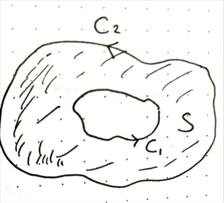
(a) Consider a vector function with the property $\nabla \times \mathbf{F} = 0$ everywhere on two closed curves $C_1$ and $C_2$ and on any capping surface $S$ of the region enclosed by them. Show that the circulation of $\mathbf{F}$ around $C_1$ equals the circulation of $\mathbf{F}$ around $C_2$.
Solution. Click to Expand
Form $C_3$ by joining $C_1$ and $C_2$ with a segment on $S$ and reversing the direction of $C_1$.
In figure below $a$ and $b$ segments completely overlap but in opposite directions. They connect inner and outer parts of the curve by moving along $S$.
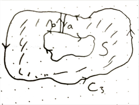
Then $S$ is a capping surface for the region enclosed by $C_3$.
Then, we have:
$$ \oint_{C_3} \mathbf{F} \cdot \hat{\mathbf{t}} \, ds = \iint_S \nabla \times \mathbf{F} \cdot \hat{\mathbf{n}} \, dS $$
Since $\nabla \times \mathbf{F} = 0$, we have:
$$ \oint_{C_3} \mathbf{F} \cdot \hat{\mathbf{t}} \, ds = 0 \tag{1} $$
Since we have reversed the direction of $C_1$ and line integrals along $a$ and $b$ cancel each other, we have:
$$ \oint_{C_3} \mathbf{F} \cdot \hat{\mathbf{t}} \, ds = -\oint_{C_1} \mathbf{F} \cdot \hat{\mathbf{t}} \, ds + \oint_{C_2} \mathbf{F} \cdot \hat{\mathbf{t}} \, ds \tag{2} $$
Putting (1) and (2) together, we have:
$$ -\oint_{C_1} \mathbf{F} \cdot \hat{\mathbf{t}} \, ds + \oint_{C_2} \mathbf{F} \cdot \hat{\mathbf{t}} \, ds = 0 $$
Thus, we have:
$$ \oint_{C_1} \mathbf{F} \cdot \hat{\mathbf{t}} \, ds = \oint_{C_2} \mathbf{F} \cdot \hat{\mathbf{t}} \, ds $$
(b) The magentic field due to an infinitely long straight wire carrying a uniform current $I$ is $\mathbf{B} = (\mu_0 I / 2 \pi r) \hat{\mathbf{e}_\theta}$. Show that $\nabla \times \mathbf{B} = 0$ everywhere except at $r = 0$.
Solution. Click to Expand
$$ \begin{align*} (\nabla \times \mathbf{B})_r &= \frac{1}{r} \frac{\partial F_z}{\partial \theta} - \frac{\partial F_\theta}{\partial z} \\[0.8em] &= - \frac{\partial}{\partial z} \left( \frac{\mu_0 I}{2 \pi r} \right) \\[0.5em] &= 0 \\[1.5em] (\nabla \times \mathbf{B})_\theta &= \frac{\partial F_r}{\partial z} - \frac{\partial F_z}{\partial r} \\[0.5em] &= 0 \\[1.5em] (\nabla \times \mathbf{B})_z &= \frac{1}{r} \frac{\partial}{\partial r}(r F_\theta) - \frac{\partial F_r}{\partial \theta} \\[1em] &= \frac{1}{r} \frac{\partial}{\partial r} \left( r \frac{\mu_0 I}{2 \pi r} \right)\\[1em] &= \frac{1}{r} \frac{\partial}{\partial r} \left( \frac{\mu_0 I}{2 \pi} \right) \\[0.5em] &= 0 \end{align*} $$
(c) Prove Ampere’s circuital law for the field of the wire given in part (b).
Solution. Click to Expand
For a circle of radius $r$, $ds = r \\, d\theta$ and $\hat{\mathbf{t}} = \hat{\mathbf{e}_\theta}$. Then, we have:
$$ \oint_{circle} \mathbf{B} \cdot \hat{\mathbf{t}} \, ds = \int_{0}^{2 \pi} \frac{\mu_0 I}{2 \pi r} r \, d\theta = \mu_0 I $$
For any curve $C$ not passing through the wire, there exists a circle around the wire inside it. Putting together the results from part (a) and (b), circulation of $\mathbf{B}$ around $C$ is equal to the circulation of $\mathbf{B}$ around the circle, which is $\mu_0 I$.
So, for any curve $C$ not passing through the wire, we have:
$$ \oint_C \mathbf{B} \cdot \hat{\mathbf{t}} \, ds = \mu_0 I $$
Problem III-18. The electromotive force $\mathcal{E}$ in a circuit $C$ is equal to the circulation of the electric field $\mathbf{E}$ around the circuit:
$$ \mathcal{E} = \oint_C \mathbf{E} \cdot \hat{\mathbf{t}} \, ds $$
Faraday discovered that in a stationary circuit an electromotive force is induced by a changing magnetic flux. That is,
$$ \mathcal{E} = - \frac{d \Phi}{dt} $$
where
$$ \Phi = \iint_S \mathbf{B} \cdot \hat{\mathbf{n}} \, dS $$
$t$ is time (don’t confuse it with the tangent vector $\hat{\mathbf{t}}$) and $S$ is any capping surface of $C$. Use this information and Stokes’ theorem to derive the equation
$$ \nabla \times \mathbf{E} = - \frac{\partial \mathbf{B}}{\partial t} $$
which is one of Maxwell’s equations.
Solution. Click to Expand
Since $\mathcal{E} = \oint_C \mathbf{E} \cdot \hat{\mathbf{t}} \\, ds$, then for any capping surface $S$ of $C$, we have:
$$ \mathcal{E} = \iint_S \nabla \times \mathbf{E} \cdot \hat{\mathbf{n}} \, dS \tag{1} $$
Differentiating $\Phi = \iint_S \mathbf{B} \cdot \hat{\mathbf{n}} \\, dS$ with respect to $t$, we have:
$$ \frac{d \Phi}{d t} = \iint_S \frac{\partial \mathbf{B}}{\partial t} \cdot \hat{\mathbf{n}} \, dS $$
Where we used the fact that $S$ is stationary, so $\hat{\mathbf{n}}$ does not depend on $t$.
From the problem statement we know that $\mathcal{E} = - \dfrac{d \Phi}{dt}$. Then, we have:
$$ \mathcal{E} = - \iint_S \frac{\partial \mathbf{B}}{\partial t} \cdot \hat{\mathbf{n}} \, dS \tag{2} $$
Putting (1) and (2) together, we have:
$$ \iint_S \nabla \times \mathbf{E} \cdot \hat{\mathbf{n}} \, dS = - \iint_S \frac{\partial \mathbf{B}}{\partial t} \cdot \hat{\mathbf{n}} \, dS $$
Since this is true for any capping surface $S$ of $C$, we have:
$$ \nabla \times \mathbf{E} = - \frac{\partial \mathbf{B}}{\partial t} $$
Problem III-19. Determine the value of the line integral $\int_C \mathbf{F} \cdot \hat{\mathbf{t}} \\, ds$, where
$$ \mathbf{F} = (e^{-y} - z e^{-x}) \mathbf{i} + (e^{-z} - x e^{-y}) \mathbf{j} + (e^{-x} - y e^{-z}) \mathbf{k} $$
and $C$ is the path
$$ \begin{cases} x = \dfrac{1}{\ln 2} \ln(1 + p), \\ y = \sin\left(\dfrac{\pi p}{2}\right), \\ z = \dfrac{1 - e^p}{1 - e}, \end{cases} \quad 0 \leq p \leq 1 $$
from $(0, 0, 0)$ to $(1, 1, 1)$.
Solution. Click to Expand
Since $\nabla \times \mathbf{F} = 0$, the line integral is independent of the path taken.
Then we can use:
- $C_1$: straight segment from $(0, 0, 0)$ to $(1, 0, 0)$,
- $C_2$: straight segment from $(1, 0, 0)$ to $(1, 1, 0)$,
- $C_3$: straight segment from $(1, 1, 0)$ to $(1, 1, 1)$.
Then we have:
$$ \begin{align*} \int_{C_1} \mathbf{F} \cdot \hat{\mathbf{t}} \, ds &= \int_{0}^{1} e^0 \, dx = 1 \\[1em] \int_{C_2} \mathbf{F} \cdot \hat{\mathbf{t}} \, ds &= \int_{0}^{1} (1 - e^{-y}) \, dy = e^{-1} \\[1em] \int_{C_3} \mathbf{F} \cdot \hat{\mathbf{t}} \, ds &= \int_{0}^{1} (e^{-1} - e^{-z}) \, dz = 2 e^{-1} - 1 \end{align*} $$
Then, we have:
$$ \int_C \mathbf{F} \cdot \hat{\mathbf{t}} \, ds = \int_{C_1 + C_2 + C_3} \mathbf{F} \cdot \hat{\mathbf{t}} \, ds = 3 e^{-1} $$
Problem III-20. Maxwell’s equations are:
$$ \begin{align*} \nabla \cdot \mathbf{E} &= \frac{\rho}{\varepsilon_0} \tag{M1} \\ \nabla \cdot \mathbf{B} &= 0 \tag{M2} \\ \nabla \times \mathbf{E} &= - \frac{\partial \mathbf{B}}{\partial t} \tag{M3} \\ \nabla \times \mathbf{B} &= \varepsilon_0 \mu_0 \frac{\partial \mathbf{E}}{\partial t} + \mu_0 \mathbf{J} \tag{M4} \end{align*} $$
where $\mathbf{E}$ is the electric field, $\mathbf{B}$ is the magnetic field, $\rho$ is the charge density, and $\mathbf{J}$ is the current density. Use Maxwell’s equations to derive the continuity equation
$$ \nabla \cdot \mathbf{J} + \frac{\partial \rho}{\partial t} = 0 $$
Solution. Click to Expand
Lemma. $\dfrac{\partial}{\partial t} \left( \nabla \cdot \mathbf{E} \right) = \nabla \cdot \left( \dfrac{\partial \mathbf{E}}{\partial t} \right)$.
Proof of Lemma. Let $\mathbf{E} = (E_x, E_y, E_z)$. Then
$$ \nabla \cdot \mathbf{E} = \dfrac{\partial E_x}{\partial x} + \dfrac{\partial E_y}{\partial y} + \dfrac{\partial E_z}{\partial z} $$
Differentiating with respect to $t$, we have:
$$ \begin{align*} \dfrac{\partial}{\partial t} \left( \nabla \cdot \mathbf{E} \right) &= \dfrac{\partial^2 E_x}{\partial x \partial t} + \dfrac{\partial^2 E_y}{\partial y \partial t} + \dfrac{\partial^2 E_z}{\partial z \partial t} \\[1em] &= \nabla \cdot \left( \frac{\partial E_x}{\partial t}, \frac{\partial E_y}{\partial t}, \frac{\partial E_z}{\partial t} \right) \\[1em] &= \nabla \cdot \left( \frac{\partial \mathbf{E}}{\partial t} \right) \end{align*} $$
Proof of Continuity Equation. From (M4) we have:
$$ \mu_0 \mathbf{J} = \nabla \times \mathbf{B} - \varepsilon_0 \mu_0 \frac{\partial \mathbf{E}}{\partial t} $$
Taking the divergence of both sides and using the linearity of the divergence operator, we have:
$$ \mu_0 \left( \nabla \cdot \mathbf{J} \right) = \nabla \cdot \left( \nabla \times \mathbf{B} \right) - \varepsilon_0 \mu_0 \nabla \cdot \frac{\partial \mathbf{E}}{\partial t} $$
In III.7 we proved that $\nabla \cdot \left( \nabla \times \mathbf{B} \right) = 0$. Then, we have:
$$ \mu_0 \left( \nabla \cdot \mathbf{J} \right) = - \varepsilon_0 \mu_0 \nabla \cdot \frac{\partial \mathbf{E}}{\partial t} $$
which means:
$$ \nabla \cdot \mathbf{J} = - \varepsilon_0 \nabla \cdot \frac{\partial \mathbf{E}}{\partial t} \tag{1} $$
Differentiating (M1) with respect to $t$, we have:
$$ \frac{\partial}{\partial t} \left( \nabla \cdot \mathbf{E} \right) = \frac{1}{\varepsilon_0} \frac{\partial \rho}{\partial t} $$
Using the lemma, we have:
$$ \nabla \cdot \frac{\partial \mathbf{E}}{\partial t} = \frac{1}{\varepsilon_0} \frac{\partial \rho}{\partial t} \tag{2} $$
Putting (1) and (2) together, we have:
$$ \nabla \cdot \mathbf{J} = - \frac{\partial \rho}{\partial t} $$
Rearranging, we have:
$$ \nabla \cdot \mathbf{J} + \frac{\partial \rho}{\partial t} = 0 $$
Problem III-21. The electromagnetic field stores energy, and it is possible to show that in a volume $V$ the amount of electromagnetic energy is
$$ \iiint_V \rho_E \, dV $$
where the energy density is
$$ \rho_E = \frac{1}{2} \left( \varepsilon_0 \mathbf{E} \cdot \mathbf{E} + \mathbf{B} \cdot \mathbf{B} / \mu_0 \right) = \frac{1}{2} \left( \varepsilon_0 E^2 + \frac{B^2}{\mu_0} \right) $$
Use Maxwell’s equations to show that
$$ \frac{\partial \rho_E}{\partial t} + \nabla \cdot \left( \frac{\mathbf{E} \times \mathbf{B}}{\mu_0} \right) = - \mathbf{J} \cdot \mathbf{E} $$
Solution. Click to Expand
Lemma. $\nabla \cdot \left( \mathbf{E} \times \mathbf{B} \right) = \mathbf{B} \cdot \left( \nabla \times \mathbf{E} \right) - \mathbf{E} \cdot \left( \nabla \times \mathbf{B} \right)$.
Proof of Lemma. We have
$$ \mathbf{E} \times \mathbf{B} = (E_y B_z - E_z B_y, E_z B_x - E_x B_z, E_x B_y - E_y B_x) $$
Then
$$ \begin{align*} \nabla \cdot \left( \mathbf{E} \times \mathbf{B} \right) &= E_y \frac{\partial B_z}{\partial x} + B_z \frac{\partial E_y}{\partial x} - E_z \frac{\partial B_y}{\partial x} - B_y \frac{\partial E_z}{\partial x} + \\ &+ E_z \frac{\partial B_x}{\partial y} + B_x \frac{\partial E_z}{\partial y} - E_x \frac{\partial B_z}{\partial y} - B_z \frac{\partial E_x}{\partial y} + \\ &+ E_x \frac{\partial B_y}{\partial z} + B_y \frac{\partial E_x}{\partial z} - E_y \frac{\partial B_x}{\partial z} - B_x \frac{\partial E_y}{\partial z} \end{align*} $$
Rearranging, we have:
$$ \begin{align*} \nabla \cdot \left( \mathbf{E} \times \mathbf{B} \right) &= E_x \left(\frac{\partial B_y}{\partial z} - \frac{\partial B_z}{\partial y}\right) + E_y \left(\frac{\partial B_z}{\partial x} - \frac{\partial B_x}{\partial z}\right) + \\ &+ E_z \left(\frac{\partial B_x}{\partial y} - \frac{\partial B_y}{\partial x}\right) + B_x \left(\frac{\partial E_z}{\partial y} - \frac{\partial E_y}{\partial z}\right) + \\ &+ B_y \left(\frac{\partial E_x}{\partial z} - \frac{\partial E_z}{\partial x}\right) + B_z \left(\frac{\partial E_y}{\partial x} - \frac{\partial E_x}{\partial y}\right) \end{align*} $$
Which can be rewritten as $B \cdot \left( \nabla \times \mathbf{E} \right) - E \cdot \left( \nabla \times \mathbf{B} \right)$.
Proof of Energy Density Equation.
Inner product of sides of (M3) by $\mathbf{B}$ on the left gives:
$$ \mathbf{B} \cdot (\nabla \times \mathbf{E}) = - \mathbf{B} \cdot \frac{\partial \mathbf{B}}{\partial t} \tag{1} $$
Inner product of sides of (M4) by $E$ on the left gives:
$$ \mathbf{E} \cdot (\nabla \times \mathbf{B}) = \varepsilon_0 \mu_0 \mathbf{E} \cdot \frac{\partial \mathbf{E}}{\partial t} + \mu_0 \mathbf{E} \cdot \mathbf{J} \tag{2} $$
Putting the lemma with (1) and (2) gives:
$$ \nabla \left( \frac{\mathbf{E} \times \mathbf{B}}{\mu_0} \right) = -\frac{1}{\mu_0} \mathbf{B} \cdot \frac{\partial \mathbf{B}}{\partial t} - \varepsilon_0 \mathbf{E} \cdot \frac{\partial \mathbf{E}}{\partial t} - \mathbf{E} \cdot \mathbf{J} \tag{3} $$
On the other hand, differentiating sides of $\rho_E = \dfrac{1}{2}(\varepsilon_0 \mathbf{E} \cdot \mathbf{E} + \mathbf{B} \cdot \mathbf{B} / \mu_0)$ with respect to $t$ gives:
$$ \frac{\partial \rho_E}{\partial t} = \frac{1}{\mu_0} \frac{\partial \mathbf{B}}{\partial t} \mathbf{B} + \varepsilon_0 \frac{\partial \mathbf{E}}{\partial t} \mathbf{E} \tag{4} $$
Putting (3) and (4) together we get:
$$ \frac{\partial \rho_E}{\partial t} + \nabla \cdot \left( \frac{\mathbf{E} \times \mathbf{B}}{\mu_0} \right) = - \mathbf{J} \cdot \mathbf{E} $$
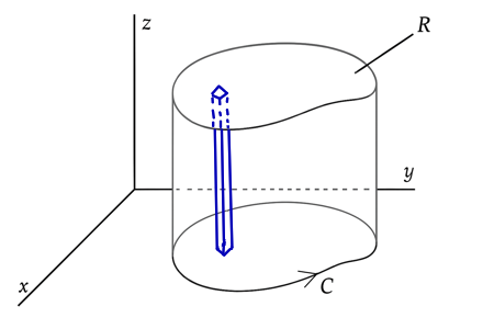
Problem III-22. (a) Apply the divergence theorem to the function
$$ \mathbf{G}(x, y) = \mathbf{i} G_x(x, y) + \mathbf{j} G_y(x, y) $$
using for $V$ and $S$ the volume and surface shown in the diagram.
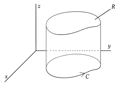
In this way obtain the relation
$$ \oint_C G_x \, dy - G_y \, dx = \iint_R \left( \frac{\partial G_x}{\partial x} + \frac{\partial G_y}{\partial y} \right) \, dx dy $$
which is the divergence theorem in two dimensions.
Solution. Click to Expand
We’ll use the divergence theorem:
$$ \iint_S \mathbf{G} \cdot \hat{\mathbf{n}} \, dS = \iiint_V \nabla \cdot \mathbf{G} \, dV \tag{1} $$
Calculating the surface integral.
First we calculate the surface integral $\iint_S \mathbf{G} \cdot \hat{\mathbf{n}} \\, dS$.
In upper and lower parts of the surface, the normal vector is $\pm \mathbf{k}$, and since $\mathbf{G}$ has $0$ as the $\mathbf{k}$ component, then the surface integral is zero.
To calculate the surface integral of the shaded part in the figure, since the value of $\mathbf{G}$ and the normal vector $\hat{\mathbf{n}}$ do not depend on the $z$-coordinate, we choose $dS$ as below. Then, $dS = h \\, ds$, where $h$ is the height of the surface.
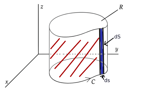
Then surface integral of the shaded part in the figure will be equal to:
$$ h \, \oint_C \mathbf{G} \cdot \hat{\mathbf{n}} \, ds $$
Since $C$ is on the $xy$-plane, then its tangent vector is:
$$ \hat{\mathbf{t}} = \mathbf{i} \frac{dx}{ds} + \mathbf{j} \frac{dy}{ds} $$
Given that $C$ is oriented counterclockwise, then the normal vector is the tangent vector rotated by $90^\circ$ clockwise:
$$ \hat{\mathbf{n}} = \mathbf{i} \frac{dy}{ds} - \mathbf{j} \frac{dx}{ds} $$
Then, we have:
$$ \begin{align*} \oint_C \mathbf{G} \cdot \hat{\mathbf{n}} \, ds &= \oint_C \left( G_x \frac{dy}{ds} - G_y \frac{dx}{ds} \right) \, ds \\[0.8em] &= \oint_C G_x \, dy - G_y \, dx \end{align*} $$
and then the total surface integral is:
$$ \iint_S \mathbf{G} \cdot \hat{\mathbf{n}} \, dS = h \oint_C G_x \, dy - G_y \, dx \tag{2} $$
Calculating the volume integral.
Since value of $\mathbf{G}$ doesn’t depend on $z$, we can choose $dV$ as below. Then, $dV = h \\, dS$.
Then, we have:
$$ \begin{align*} \iiint_V \nabla \cdot \mathbf{G} \, dV &= h \iint_R \nabla \cdot \mathbf{G} \, dS \\[0.8em] &= h \iint_R \left( \frac{\partial G_x}{\partial x} + \frac{\partial G_y}{\partial y} \right) \, dx dy \tag{3} \end{align*} $$
Finally, putting (1), (2), and (3) together, we have:
$$ \oint_C G_x \, dy - G_y \, dx = \iint_R \left( \frac{\partial G_x}{\partial x} + \frac{\partial G_y}{\partial y} \right) \, dx dy $$
(b) Apply Stokes’ theorem to the function
$$ \mathbf{F}(x, y) = \mathbf{i} F_x(x, y) + \mathbf{j} F_y(x, y) $$
using for $C$ a closed curve lying entirely in the $xy$-plane and for $S$ the region $R$ of the $xy$-plane enclosed by $C$. In this way obtain the relation
$$ \oint_C F_x \, dx + F_y \, dy = \iint_R \left( \frac{\partial F_y}{\partial x} - \frac{\partial F_x}{\partial y} \right) \, dx dy $$
which is Stokes’ theorem in two dimensions.
Solution. Click to Expand
Since $S$ lies entirely in the $xy$-plane, then
- Assuming counterclockwise orientation, $\hat{\mathbf{n}} = \hat{\mathbf{k}}$,
- $dS = dx \\, dy$.
Since $\nabla \times \mathbf{F} = \mathbf{k} \left( \dfrac{\partial F_y}{\partial x} - \dfrac{\partial F_x}{\partial y} \right)$, we have:
$$ \nabla \times \mathbf{F} \cdot \hat{\mathbf{n}} = \frac{\partial F_y}{\partial x} - \frac{\partial F_x}{\partial y} $$
and then:
$$ \iint_S \nabla \times \mathbf{F} \cdot \hat{\mathbf{n}} \, dS = \iint_R \left( \frac{\partial F_y}{\partial x} - \frac{\partial F_x}{\partial y} \right) \, dx dy \tag{1} $$
Since $C$ is a closed curve lying entirely in the $xy$-plane, then:
$$ \oint_C \mathbf{F} \cdot \hat{\mathbf{t}} \, ds = \oint_C F_x \, dx + F_y \, dy \tag{2} $$
Then, by Stokes’ theorem we have:
$$ \oint_C \mathbf{F} \cdot \hat{\mathbf{t}} \, ds = \iint_S \nabla \times \mathbf{F} \cdot \hat{\mathbf{n}} \, dS \tag{3} $$
Putting (1), (2), and (3) together, we have:
$$ \oint_C F_x \, dx + F_y \, dy = \iint_R \left( \frac{\partial F_y}{\partial x} - \frac{\partial F_x}{\partial y} \right) \, dx dy $$
(c) Show that in two dimensions the divergence theorem and Stokes’ theorem are identical.
Solution. Click to Expand
The divergence theorem for $\mathbf{i} F_x + \mathbf{j} F_y$ is the same as Stokes’ theorem for $-\mathbf{i} F_y + \mathbf{j} F_x$.
So they are identical in two dimensions.
Problem III-23. (a) Let $C$ be a closed curve lying in the $xy$-plane. What condition must the function $\mathbf{F}$ satisfy in order that
$$ \oint_C \mathbf{F} \cdot \hat{\mathbf{t}} \, ds = A $$
where $A$ is the area enclosed by $C$?
Solution. Click to Expand
Using the 2-dimensional Stokes’ theorem, we have:
$$ \oint_C F_x \, dx + F_y \, dy = \iint_R \left( \frac{\partial F_y}{\partial x} - \frac{\partial F_x}{\partial y} \right) \, dx \, dy $$
So, in order for the line integral to be equal to the area enclosed by $C$, we need:
$$ \frac{\partial F_y}{\partial x} - \frac{\partial F_x}{\partial y} = 1 $$
or equivalently:
$$ \nabla \times \mathbf{F} = \mathbf{k} $$
(b) Give some examples of functions $\mathbf{F}$ having the property described in part (a).
Solution. Click to Expand
- $\mathbf{F} = \mathbf{i} y + 2 \mathbf{j} x$
- $\mathbf{F} = \hat{\mathbf{e}}_\theta \dfrac{r}{2}$ (cylendrical coordinates)
(c) Use line integrals to find formulas for the area of
- a rectangle
- a right triangle
- a circle
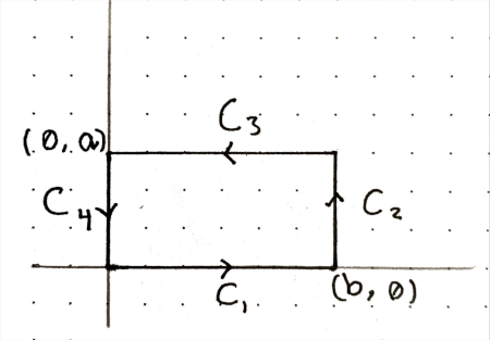
A Rectangle. Click to Expand
Let $\mathbf{F} = \mathbf{i} y + 2 \mathbf{j} x$ and consider the rectangle below:
Then, we have:
$$ \begin{align*} \int_{C_1} \mathbf{F} \cdot \hat{\mathbf{t}} \, ds &= 0 \\[0.8em] \int_{C_2} \mathbf{F} \cdot \hat{\mathbf{t}} \, ds &= \int_{0}^{a} 2 \cdot b \, dy = 2 a b \\[0.8em] \int_{C_3} \mathbf{F} \cdot \hat{\mathbf{t}} \, ds &= \int_{b}^{0} a \, dx = - a b \\[0.8em] \int_{C_4} \mathbf{F} \cdot \hat{\mathbf{t}} \, ds &= 0 \end{align*} $$
Putting together, we have:
$$ \oint_{C_1 + C_2 + C_3 + C_4} \mathbf{F} \cdot \hat{\mathbf{t}} \, ds = 2 a b - a b = a b $$
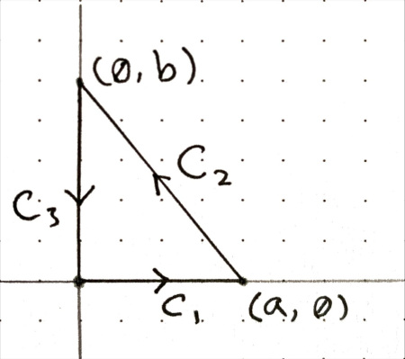
A Right Triangle. Click to Expand
Let $\mathbf{F} = \mathbf{i} y + 2 \mathbf{j} x$ and consider the right triangle below:
Then, we have:
$$ \begin{align*} \int_{C_1} \mathbf{F} \cdot \hat{\mathbf{t}} \, ds &= 0 \\[0.8em] \int_{C_3} \mathbf{F} \cdot \hat{\mathbf{t}} \, ds &= 0 \end{align*} $$
For $C_2$, note that $y = \dfrac{b}{a} (a - x)$, so $dy = -\dfrac{b}{a} \\, dx$.
Then, we have:
$$ \begin{align*} \int_{C_2} \mathbf{F} \cdot \hat{\mathbf{t}} \, ds &= \int_{C_2} (y \, dx + 2 x \, dy) \\[0.8em] &= \int_{0}^{a} \left( \dfrac{b}{a} (a - x) \, dx - 2 x \dfrac{b}{a} \, dx \right) \\[0.8em] &= \int_{0}^{a} \left( \dfrac{b}{a} (a - 3 x) \right) \, dx \\[0.8em] &= \frac{ab}{2} \end{align*} $$
A Circle. Click to Expand
Let $\mathbf{F} = \hat{\mathbf{e}}_\theta \dfrac{r}{2}$. We have $ds = r \\, d\theta$ and $\hat{\mathbf{t}} = \hat{\mathbf{e}}_\theta$.
Then, we have:
$$ \begin{align*} \oint_C \mathbf{F} \cdot \hat{\mathbf{t}} \, ds &= \oint_C \left( \frac{r}{2} \right) r \, d\theta \\[0.8em] &= \frac{r^2}{2} \int_0^{2\pi} \, d\theta = \pi r^2 \end{align*} $$
(d) Show that the area enclosed by the plane curve $C$ is the magnitude of
$$ \frac{1}{2} \oint_C \mathbf{r} \times \hat{\mathbf{t}} \, ds $$
where $\mathbf{r} = \mathbf{i} x + \mathbf{j} y$.
Solution. Click to Expand
We have $\hat{\mathbf{t}} = \mathbf{i} \dfrac{dx}{ds} + \mathbf{j} \dfrac{dy}{ds}$, then:
$$ \begin{align*} \mathbf{r} \times \hat{\mathbf{t}} &= \mathbf{k} \left( x \frac{dy}{ds} - y \frac{dx}{ds} \right) \\[0.8em] &= \mathbf{k} \left( (-y \mathbf{i} + x \mathbf{j}) \cdot \hat{\mathbf{t}} \right) \end{align*} $$
Then, we have:
$$ \frac{1}{2} \oint_C \mathbf{r} \times \hat{\mathbf{t}} \, ds = \frac{\mathbf{k}}{2} \oint_C (-y \mathbf{i} + x \mathbf{j}) \cdot \hat{\mathbf{t}} \, ds $$
Since $\nabla \times (-y \mathbf{i} + x \mathbf{j}) = 2 \mathbf{k}$, then by Stokes’ theorem we have:
$$ \oint_C (-y \mathbf{i} + x \mathbf{j}) \cdot \hat{\mathbf{t}} \, ds = 2 A $$
Then, we have:
$$ \frac{1}{2} \oint_C \mathbf{r} \times \hat{\mathbf{t}} \, ds = A \mathbf{k} $$
which has a magnitude of $A$.
Problem III-24. (a) There is an important theorem in vector calculus that says $\nabla \cdot \mathbf{G} = 0$ if and only if $\mathbf{G} = \nabla \times \mathbf{H}$. To prove this we note first of all that $\mathbf{G} = \nabla \times \mathbf{H}$ implies $\nabla \cdot \mathbf{G} = 0$ (see problem III-7).
To show that $\nabla \cdot \mathbf{G} = 0$ implies $\mathbf{G} = \nabla \times \mathbf{H}$, the simplest procedure is to give $\mathbf{H}$:
$$ \begin{align*} H_x &= 0 \\[1em] H_y &= \int_{x_0}^{x} G_z(x', y, z) \, dx' \\[1em] H_z &= - \int_{x_0}^{x} G_y(x', y, z) \, dx' + \int_{y_0}^{y} G_x(x_0, y', z) \, dy' \end{align*} $$
where $x_0$ and $y_0$ are arbitrary constants. Show by direct calculation that if $\nabla \cdot \mathbf{G} = 0$, then $\mathbf{G} = \nabla \times \mathbf{H}$.
Solution. Click to Expand
Since $\nabla \cdot \mathbf{G} = 0$, then:
$$ \frac{\partial G_x}{\partial x} = - \frac{\partial G_y}{\partial y} - \frac{\partial G_z}{\partial z} \tag{1} $$
We have:
$$ \begin{align*} \nabla \times \mathbf{H} &= \mathbf{i} \left( \frac{\partial H_z}{\partial y} - \frac{\partial H_y}{\partial z} \right) + \mathbf{j} \left( \frac{\partial H_x}{\partial z} - \frac{\partial H_z}{\partial x} \right) + \mathbf{k} \left( \frac{\partial H_y}{\partial x} - \frac{\partial H_x}{\partial y} \right) \\[1em] &= \mathbf{i} \left( \frac{\partial H_z}{\partial y} - \frac{\partial H_y}{\partial z} \right) \+ \mathbf{j} \left( 0 - \frac{\partial H_z}{\partial x} \right) + \mathbf{k} \left( \frac{\partial H_y}{\partial x} - 0 \right) \end{align*} $$
We have:
$$ \begin{align*} \frac{\partial H_y}{\partial x} &= G_z(x, y, z) \\[1em] \frac{\partial H_y}{\partial z} &= \int_{x_0}^{x} \frac{\partial G_z(x', y, z)}{\partial z} \, dx' \\[1em] \frac{\partial H_z}{\partial x} &= - G_y(x, y, z) \\[1em] \frac{\partial H_z}{\partial y} &= - \int_{x_0}^{x} \frac{\partial G_y(x', y, z)}{\partial y} \, dx' + G_x(x_0, y, z) \end{align*} $$
As a direct consequence, we have:
$$ \begin{align*} (\nabla \times \mathbf{H})_y &= G_y(x, y, z) \\[1em] (\nabla \times \mathbf{H})_z &= G_z(x, y, z) \end{align*} $$
To calculate $(\nabla \times \mathbf{H})_x$, we have:
$$ (\nabla \times \mathbf{H})_x = \int_{x_0}^{x} \left( - \frac{\partial G_y(x', y, z)}{\partial y} - \frac{\partial G_z(x', y, z)}{\partial z} \right) \, dx' + G_x(x_0, y, z) $$
Using (1), we have:
$$ (\nabla \times \mathbf{H})_x = \int_{x_0}^{x} \frac{\partial G_x(x', y, z)}{\partial x} \, dx' + G_x(x_0, y, z) $$
Then using the fundamental theorem of calculus, we have:
$$ (\nabla \times \mathbf{H})_x = G_x(x, y, z) - G_x(x_0, y, z) + G_x(x_0, y, z) = G_x(x, y, z) $$
(b) Is the vector function $\mathbf{H}$ specified in part (a) unique? That is, can we alter it in any way without invalidating the relation $\mathbf{G} = \nabla \times \mathbf{H}$?
Solution. Click to Expand
No, the vector function $\mathbf{H}$ is not unique. For example, adding constants to the components of $\mathbf{H}$ does not change the value of $\nabla \times \mathbf{H}$.
Problem III-25. Determine in which of the following cases it is possible to write $\mathbf{G} = \nabla \times \mathbf{H}$. In the cases where it is possible, find $\mathbf{H}$.
(a) $\mathbf{G} = \mathbf{i} x + \mathbf{j} y + \mathbf{k} z$
Solution Click to Expand
Possible, since $\nabla \cdot \mathbf{G} = 0$.
Using the formula from Problem III-24(a), we have:
$$ \mathbf{H} = \mathbf{j} \frac{x^2 - x_0^2}{2} + \mathbf{k} \left( -z (x - x_0) + \frac{y^2 - y_0^2}{2} \right) $$
For any $x_0$ and $y_0$.
(b) $\mathbf{G} = B_0 \mathbf{k}$, where $B_0$ is a constant
Solution Click to Expand
Possible, since $\nabla \cdot \mathbf{G} = 0$.
Using the formula from Problem III-24(a), we have:
$$ \mathbf{H} = \mathbf{j} B_0 (x - x_0) $$
for any $x_0$.
(c) $\mathbf{G} = \mathbf{i} x^2 - \mathbf{k} y^2$
Solution Click to Expand
Not possible, since $\nabla \cdot \mathbf{G} = 2x \neq 0$.
(d) $\mathbf{G} = 2 \mathbf{i} x - \mathbf{j} y - \mathbf{k} z$
Solution Click to Expand
Possible, since $\nabla \cdot \mathbf{G} = 0$.
Using the formula from Problem III-24(a), we have:
$$ \mathbf{H} = -\mathbf{j} z (x - x_0) + \mathbf{k} \left( x y + x_0 y - 2 x_0 y_0 \right) $$
For any $x_0$ and $y_0$.
(e) $\mathbf{G} = 2 \mathbf{i} x - \mathbf{j} y + \mathbf{k} z$
Solution Click to Expand
Not possible, since $\nabla \cdot \mathbf{G} = 2 \neq 0$.
Problem III-26. Since the divergence of any magnetic field $\mathbf{B}$ is zero, we can write $\mathbf{B} = \nabla \times \mathbf{A}$. Prove that the circulation of $\mathbf{A}$ around any closed path $C$ is equal to the flux of $\mathbf{B}$ through any surface $S$ capping $C$.
Solution. Click to Expand
$$ \begin{align*} \oint_C \mathbf{A} \cdot \hat{\mathbf{t}} \, ds &= \iint_S (\nabla \times \mathbf{A}) \cdot \hat{\mathbf{n}} \, dS \quad \text{(Stokes' Theorem)} \\[1em] &= \iint_S \mathbf{B} \cdot \hat{\mathbf{n}} \, dS \\[1em] \end{align*} $$
which is the flux of $\mathbf{B}$ through $S$.
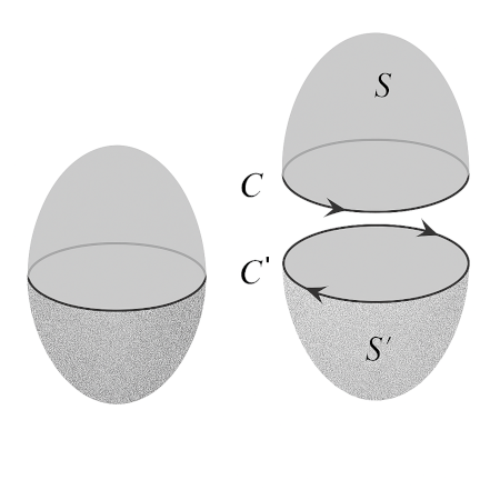
Problem III-27. Prove the statement made in Problem III-24(a) by applying Stokes’ theorem and divergence theorem. [Hint: See the diagram below]
Solution. Click to Expand
Assume that $\mathbf{G} = \nabla \times \mathbf{H}$.
For any closed surface $S$ capping $C$ and $S'$ capping $C'$, let $V$ be the volume enclosed by $S$ and $S'$. Then, we have:
$$ \begin{align*} \iiint_V \nabla \cdot \mathbf{G} \, dV &= \iint_{S+S'} \mathbf{G} \cdot \hat{\mathbf{n}} \, dS &\text{(Divergence Theorem)} \\[1em] &= \iint_{S+S'} (\nabla \times \mathbf{H}) \cdot \hat{\mathbf{n}} \, dS \\[1em] &= \oint_{C + C'} \mathbf{H} \cdot \hat{\mathbf{t}} \, ds &\text{(Stokes' Theorem)} \end{align*} $$
Since $C$ and $C'$ follow the same path but in opposite directions, then the last integral is zero.
So, for volume bounded by any $S$ and $S'$ capping $C$ and $C'$, we have:
$$ \iiint_V \nabla \cdot \mathbf{G} \, dV = 0 $$
Since choice of $S$ and $S'$ is arbitrary, it implies that $\nabla \cdot \mathbf{G} = 0$.
Problem III-28. (a) What is the integral form of the equation $\mathbf{G} = \nabla \times \mathbf{H}$?
Solution. Click to Expand
Using the Stokes’ theorem, for a closed path $C$ and a surface $S$ capping $C$, we have:
$$ \iint_S \nabla \times \mathbf{H} \cdot \hat{\mathbf{n}} \, dS = \oint_C \mathbf{H} \cdot \hat{\mathbf{t}} \, ds $$
Since $\mathbf{G} = \nabla \times \mathbf{H}$, then we have:
$$ \iint_S \mathbf{G} \cdot \hat{\mathbf{n}} \, dS = \oint_C \mathbf{H} \cdot \hat{\mathbf{t}} \, ds $$
and this is the integral form of the equation $\mathbf{G} = \nabla \times \mathbf{H}$.
Problem III-29.
In the text we defined the curl as the limit of a certain ratio. An alternative definition is provided by the equation
$$ \nabla \times \mathbf{F} = \lim_{\Delta V \to 0} \frac{1}{\Delta V} \iint_S \hat{\mathbf{n}} \times \mathbf{F} \, dS $$
where $\mathbf{F}$ is a vector function of position, the integration is carried out over a closed surface $S$ which encloses the volume $\Delta V$, and $\hat{\mathbf{n}}$ is the unit vector normal to $S$ pointing outward.
(a) Integrate over a “cuboid” and show that the definition given above yields Equation (III-7b).
Solution. Click to Expand
Consider the cuboid shown in the figure below:
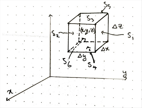
Side S1.
- Normal: $\hat{\mathbf{j}}$,
- $\hat{\mathbf{n}} \times \mathbf{F} = \hat{\mathbf{i}} F_z - \hat{\mathbf{k}} F_x$,
- Area: $dS = \Delta x \\, \Delta z$.
Then, we have:
$$ \iint_{S_1} \hat{\mathbf{n}} \times \mathbf{F} \, dS \approx \Delta x \Delta z \left( \mathbf{i} F_z(x, y + \frac{\Delta y}{2}, z) - \mathbf{k} F_x(x, y + \frac{\Delta y}{2}, z) \right) $$
Then:
$$ \frac{1}{\Delta V} \iint_{S_1} \hat{\mathbf{n}} \times \mathbf{F} \, dS \approx \frac{\mathbf{i} F_z(x, y + \frac{\Delta y}{2}, z) - \mathbf{k} F_x(x, y + \frac{\Delta y}{2}, z)}{\Delta y} $$
Side S2.
- Normal: $-\hat{\mathbf{j}}$,
- $\hat{\mathbf{n}} \times \mathbf{F} = -\hat{\mathbf{i}} F_z + \hat{\mathbf{k}} F_x$,
- Area: $dS = \Delta x \\, \Delta z$.
Then, we have:
$$ \iint_{S_2} \hat{\mathbf{n}} \times \mathbf{F} \, dS \approx -\Delta x \Delta z \left( \mathbf{i} F_z(x, y - \frac{\Delta y}{2}, z) - \mathbf{k} F_x(x, y - \frac{\Delta y}{2}, z) \right) $$
Then:
$$ \frac{1}{\Delta V} \iint_{S_2} \hat{\mathbf{n}} \times \mathbf{F} \, dS \approx -\frac{\mathbf{i} F_z(x, y - \frac{\Delta y}{2}, z) - \mathbf{k} F_x(x, y - \frac{\Delta y}{2}, z)}{\Delta y} $$
Adding S1 and S2.
$$ \begin{align*} \frac{1}{\Delta V} \iint_{S_1+S_2} &\hat{\mathbf{n}} \times \mathbf{F} \, dS \approx \\ & \mathbf{i} \frac{F_z(x, y + \frac{\Delta y}{2}, z) - F_z(x, y - \frac{\Delta y}{2}, z)}{\Delta y} \\ \- &\mathbf{k} \frac{F_x(x, y + \frac{\Delta y}{2}, z) - F_x(x, y - \frac{\Delta y}{2}, z)}{\Delta y} \end{align*} $$
which means:
$$ \lim_{\Delta V \to 0} \frac{1}{\Delta V} \iint_{S_1+S_2} \hat{\mathbf{n}} \times \mathbf{F} \, dS = \mathbf{i} \frac{\partial F_z}{\partial y} - \mathbf{k} \frac{\partial F_x}{\partial y} $$
S3 and S4. Similarly, we can show that:
$$ \lim_{\Delta V \to 0} \frac{1}{\Delta V} \iint_{S_3+S_4} \hat{\mathbf{n}} \times \mathbf{F} \, dS = \mathbf{j} \frac{\partial F_x}{\partial z} - \mathbf{i} \frac{\partial F_y}{\partial z} $$
S5 and S6. Similarly, we can show that:
$$ \lim_{\Delta V \to 0} \frac{1}{\Delta V} \iint_{S_5+S_6} \hat{\mathbf{n}} \times \mathbf{F} \, dS = \mathbf{k} \frac{\partial F_y}{\partial x} - \mathbf{j} \frac{\partial F_z}{\partial x} $$
Putting these together, we have:
$$ \begin{align*} \nabla \times \mathbf{F} &= \lim_{\Delta V \to 0} \frac{1}{\Delta V} \iint_S \hat{\mathbf{n}} \times \mathbf{F} \, dS \\[1em] &= \mathbf{i} \left(\frac{\partial F_z}{\partial y} - \frac{\partial F_y}{\partial z}\right) + \mathbf{j} \left(\frac{\partial F_x}{\partial z} - \frac{\partial F_z}{\partial x}\right) + \mathbf{k} \left(\frac{\partial F_y}{\partial x} - \frac{\partial F_x}{\partial y}\right) \end{align*} $$
(b) Arguing as we did in the text in establishing the divergence theorem, use the above expression for the curl to derive the equation
$$ \iint_S \hat{\mathbf{n}} \times \mathbf{F} \, dS = \iiint_V \nabla \times \mathbf{F} \, dV $$
Solution. Click to Expand
Assume we partition the volume $V$ into $N$ small cubes of volume $\Delta V$.
Since normal vector of overlapping sides of two adjacent cubes are equal and opposite, then $\hat{\mathbf{n}} \times \mathbf{F}$ of two overlapping sides of two adjacent cubes will cancel out.
Then, we have:
$$ \iint_S \hat{\mathbf{n}} \times \mathbf{F} \, dS = \iint_{S_1} \hat{\mathbf{n}} \times \mathbf{F} \, dS + \ldots + \iint_{S_N} \hat{\mathbf{n}} \times \mathbf{F} \, dS $$
where $S_i$ is the surface of the $i$-th cube.
Also, since we have:
$$ \nabla \times \mathbf{F}(x_i, y_i, z_i) \approx \frac{1}{\Delta V} \iint_{S_i} \hat{\mathbf{n}} \times \mathbf{F} \, dS $$
(where $(x_i, y_i, z_i)$ is the center of the $i$-th cube), then we have:
$$ (\nabla \times \mathbf{F}(x_i, y_i, z_i)) \Delta V \approx \iint_{S_i} \hat{\mathbf{n}} \times \mathbf{F} \, dS $$
Summing over all $N$ cubes and taking the limit as $\Delta V \to 0$, we have:
$$ \iiint_V \nabla \times \mathbf{F} \, dV = \iint_S \hat{\mathbf{n}} \times \mathbf{F} \, dS $$
(c) Derive the equation in part (b) directly from the divergence theorem.
Solution. Click to Expand
Expanding $\nabla \times \mathbf{F}$ gives:
$$ \begin{align*} \iiint_V \nabla &\times \mathbf{F} \, dV = \\[1em] &\mathbf{i} \iiint_V \left( \frac{\partial F_z}{\partial y} - \frac{\partial F_y}{\partial z} \right) dV + \\[1em] &\mathbf{j} \iiint_V \left( \frac{\partial F_x}{\partial z} - \frac{\partial F_z}{\partial x} \right) dV + \\[1em] &\mathbf{k} \iiint_V \left( \frac{\partial F_y}{\partial x} - \frac{\partial F_x}{\partial y} \right) dV \end{align*} $$
Which can be rewritten as:
$$ \begin{align*} \iiint_V \nabla \times \mathbf{F} \, dV &= \\[1em] &\mathbf{i} \iiint_V \nabla \cdot \left( 0, F_z, -F_y \right) \, dV + \\[1em] &\mathbf{j} \iiint_V \nabla \cdot \left(-F_z, 0, F_x \right) \, dV + \\[1em] &\mathbf{k} \iiint_V \nabla \cdot \left( F_y, -F_x, 0 \right) \, dV \end{align*} $$
Using the divergence theorem, we have:
$$ \begin{align*} \iiint_V \nabla \times \mathbf{F} \, dV &= \\[1em] &\mathbf{i} \iint_S \left( 0, F_z, -F_y \right) \cdot \hat{\mathbf{n}} \, dS + \\[1em] &\mathbf{j} \iint_S \left(-F_z, 0, F_x \right) \cdot \hat{\mathbf{n}} \, dS + \\[1em] &\mathbf{k} \iint_S \left( F_y, -F_x, 0 \right) \cdot \hat{\mathbf{n}} \, dS \end{align*} $$
which can be rewritten as:
$$ \begin{align*} \iiint_V &\nabla \times \mathbf{F} \, dV = \\[1em] &\iint_S \left( \mathbf{i} (F_z \hat{\mathbf{n}}_y - F_y \hat{\mathbf{n}}_z) + \\[1em] \mathbf{j} (-F_z \hat{\mathbf{n}}_x + F_x \hat{\mathbf{n}}_z) + \\[1em] \mathbf{k} (F_y \hat{\mathbf{n}}_x - F_x \hat{\mathbf{n}}_y) \right) \, dS \end{align*} $$
So:
$$ \iiint_V \nabla \times \mathbf{F} \, dV = \iint_S \hat{\mathbf{n}} \times \mathbf{F} \, dS $$
Problem III-30.
The result
$$ (\nabla \times \mathbf{F})_z = \frac{\partial F_y}{\partial x} - \frac{\partial F_x}{\partial y} $$
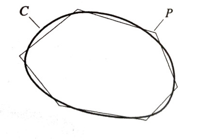
has been established by calculating the circulation of $\mathbf{F}$ around a rectangle and around a right triangle. In this problem we will show that the result holds when the circulation is calculated around any closed curve lying in the $xy$-plane.
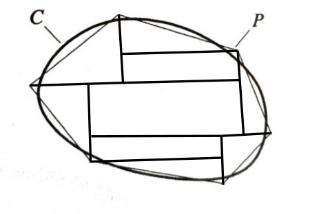
(a) Approximate an arbitrary closed curve $C$ lying in the $xy$-plane by a polygonal $P$ as shown in the figure. Subdivide the area enclosed by $P$ into $N$ patches of which the $l$-th has area $\Delta S_l$. Convince yourself by means of a sketch that this subdivision can be made with only two kinds of patches: rectangles and right triangles.
Solution. Click to Expand
Step 1. Form right triangles taking each oblique segment of $P$ as the hypotenuse.
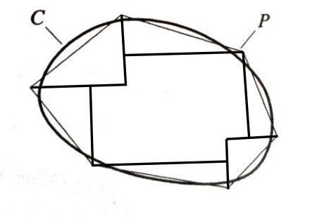
If right triangles overlap each other or the sides of $P$, then subdivide them into smaller right triangles:
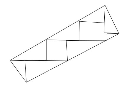
Step 2. Now, we have only right triangles and polygons with sides parallel to the axes. Add vertical segments at concave 270° corners of the polygon to form rectangles:
(b) Letting $C(x, y) = \dfrac{\partial F_y}{\partial x} - \dfrac{\partial F_x}{\partial y}$, use Taylor series to show that for $N$ large and each $\Delta S_l$ small,
$$ \begin{align*} \oint_P \mathbf{F} \cdot \hat{\mathbf{t}} \, ds &= \sum_{l=1}^N \oint_{C_l} \mathbf{F} \cdot \hat{\mathbf{t}} \, ds \\[1em] &\approx C(x_0, y_0) \Delta A + \left( \frac{\partial C}{\partial x} \right)_{x_0, y_0} \sum_{l=1}^N (x_l - x_0) \Delta S_l \\[1em] &\quad + \left( \frac{\partial C}{\partial y} \right)_{x_0, y_0} \sum_{l=1}^N (y_l - y_0) \Delta S_l + \cdots \end{align*} $$
where $C_l$ is the perimeter of the $l$-th patch, $(x_0, y_0)$ is some point in the region enclosed by $P$, and $\Delta A$ is the area enclosed by $P$.
Solution. Click to Expand
Segments in patches that are not in the perimeter of $P$ are traced twice, and in opposite directions, so they cancel out. Thus, we can write:
$$ \oint_P \mathbf{F} \cdot \hat{\mathbf{t}} \, ds = \sum_{l=1}^N \oint_{C_l} \mathbf{F} \cdot \hat{\mathbf{t}} \, ds \tag{1} $$
We can approximate the circulation around $C_l$ by:
$$ \oint_{C_l} \mathbf{F} \cdot \hat{\mathbf{t}} \, ds \approx C(x_l, y_l) \, \Delta S_l \tag{2} $$
where $(x_l, y_l)$ is the center of the $l$-th patch.
To approximate $C(x_l, y_l)$, we can use the two dimensional Taylor series.
Taylor expansion of $C(x_l, y_l)$ gives:
$$ C(x_l, y_l) \approx C(x_0, y_0) + \left( \frac{\partial C}{\partial x} \right)_{x_0, y_0} (x_l - x_0) + \left( \frac{\partial C}{\partial y} \right)_{x_0, y_0} (y_l - y_0) + \cdots \tag{3} $$
Putting (1), (2), and (3) together, we have:
$$ \begin{align*} \oint_P \mathbf{F} &\cdot \hat{\mathbf{t}} \, ds \approx \\[1em] &C(x_0, y_0) \Delta A + \left( \frac{\partial C}{\partial x} \right)_{x_0, y_0} \sum_{l=1}^N (x_l - x_0) \Delta S_l \\[1em] &\quad + \left( \frac{\partial C}{\partial y} \right)_{x_0, y_0} \sum_{l=1}^N (y_l - y_0) \Delta S_l + \cdots \end{align*} $$
(c) Show that
$$ \begin{align*} \lim_{N \to \infty} \oint_P \mathbf{F} \cdot \hat{\mathbf{t}} \, ds &= \oint_C \mathbf{F} \cdot \hat{\mathbf{t}} \, ds \\[1em] &\= \Bigl( C(x_0, y_0) + (\overline{x} - x_0) \left( \frac{\partial C}{\partial x} \right)_{x_0, y_0} \\[1em] &\+ (\overline{y} - y_0) \left( \frac{\partial C}{\partial y} \right)_{x_0, y_0} + \cdots \Bigr) \Delta S \end{align*} $$
where $\Delta S$ is the area of the region $R$ enclosed by $C$ and $(\overline{x}, \overline{y})$ is the centroid of $R$. That is:
$$ \overline{x} = \frac{1}{\Delta S} \iint_R x \, dx \, dy, \quad \overline{y} = \frac{1}{\Delta S} \iint_R y \, dx \, dy $$
Solution. Click to Expand
We have:
$$ \begin{align*} \lim_{N \to \infty} \sum_{l=1}^N (x_l - x_0) \Delta S_l &= \lim_{N \to \infty} \sum_{l=1}^N (x_l \Delta S_l) - x_0 \left( \lim_{N \to \infty} \sum_{l=1}^N \Delta S_l \right) \\[1em] &= \iint_R x \, dx \, dy - x_0 \Delta S \\[1em] &= \Delta S (\overline{x} - x_0) \end{align*} $$
Similarly, we can get:
$$ \lim_{N \to \infty} \sum_{l=1}^N (y_l - y_0) \Delta S_l = \Delta S (\overline{y} - y_0) $$
Putting this together, we have:
$$ \begin{align*} \oint_C \mathbf{F} \cdot \hat{\mathbf{t}} \, ds &= \lim_{N \to \infty} \sum_{l=1}^N \oint_{C_l} \mathbf{F} \cdot \hat{\mathbf{t}} \, ds \\[1em] &= \Bigl( C(x_0, y_0) + (\overline{x} - x_0) \left( \frac{\partial C}{\partial x} \right)_{x_0, y_0} \\[1em] &\+ (\overline{y} - y_0) \left( \frac{\partial C}{\partial y} \right)_{x_0, y_0} + \cdots \Bigr) \Delta S \end{align*} $$
(d) Finally, calculate
$$ (\nabla \times \mathbf{F})_z = \lim_{\Delta S \to 0} \frac{1}{\Delta S} \oint_P \mathbf{F} \cdot \hat{\mathbf{t}} \, ds $$
Solution. Click to Expand
As $\Delta S \to 0$, then $(\overline{x}, \overline{y}) \to (x, y)$, and we have:
$$ \begin{align*} \lim_{\Delta S \to 0} \frac{1}{\Delta S} \oint_P \mathbf{F} \cdot \hat{\mathbf{t}} \, ds &= \lim_{\Delta S \to 0} \Bigl( C(x_0, y_0) + (\overline{x} - x_0) \left( \frac{\partial C}{\partial x} \right)_{x_0, y_0} \\[1em] &\+ (\overline{y} - y_0) \left( \frac{\partial C}{\partial y} \right)_{x_0, y_0} + \cdots \Bigr) \\[1em] &= \lim_{\Delta S \to 0} C(x_l, y_l) \\[1em] &= \frac{\partial F_y}{\partial x} - \frac{\partial F_x}{\partial y} \end{align*} $$