Surface Integrals and the Divergence

Gauss’s Law

Goal: A convenient way to find the electrostatic field.

Doesn’t equations in last section already solve this? Generally, no. Unless we have very few charges and/or they are arrange simply or symmetrically. So, they’re not very useful in practice.

Which brings us to Gauss’s Law:

$$ \iint_S \mathbf{E} \cdot \hat{\mathbf{n}} \, dS = \frac{q}{\epsilon_0} \tag{II-1} $$

Here we are doing a surface integral, where integrand is the dot product of the electric field $\mathbf{E}$ and the unit normal vector $\hat{\mathbf{n}}$.

We’ll discuss these in the following sections.

The Unit Normal Vector

Let $\mathbf{u}$ and $\mathbf{v}$ be two non-collinear tangent vectors to a surface $S$ at a point $P$. A vector $\mathbf{N}$ perpendicular to both $\mathbf{u}$ and $\mathbf{v}$ is called a normal vector to $S$ at $P$.

Cross product of $\mathbf{u}$ and $\mathbf{v}$ has this property. Thus:

$$ \mathbf{\hat{n}} = \frac{\mathbf{N}}{|\mathbf{N}|} = \frac{\mathbf{u} \times \mathbf{v}}{|\mathbf{u} \times \mathbf{v}|} $$

Assume $S$ is given by the equation $z = f(x, y)$. Then parametric equation of $S$ is $\mathbf{s}(x, y) = (x, y, f(x, y))$.

Let $x$-curve be given when we hold $y$ constant and vary $x$: $\mathbf{s}(x, y_0) = (x, y_0, f(x, y_0))$. Let $y$-curve be given when we hold $x$ constant and vary $y$: $\mathbf{s}(x_0, y) = (x_0, y, f(x_0, y))$.

Then the tangent at point $P$ to the $x$-curve is $\mathbf{s}_x = \dfrac{\partial \mathbf{s}}{\partial x} = (1, 0, \dfrac{\partial f}{\partial x})$, and the tangent at point $P$ to the $y$-curve is $\mathbf{s}_y = \dfrac{\partial \mathbf{s}}{\partial y} = (0, 1, \dfrac{\partial f}{\partial y})$.

The normal vector is given by $\mathbf{N} = \mathbf{s}_x \times \mathbf{s}_y$.

Thus, the unit normal vector is given by:

$$ \begin{align*} \mathbf{\hat{n}} = \frac{\mathbf{s}_x \times \mathbf{s}_y}{|\mathbf{s}_x \times \mathbf{s}_y|} &= \frac{\left(1, 0, \dfrac{\partial f}{\partial x}\right) \times \left(0, 1, \dfrac{\partial f}{\partial y}\right)}{|\mathbf{s}_x \times \mathbf{s}_y|} \\[1em] &= \frac{-\mathbf{i}\dfrac{\partial f}{\partial x} + -\mathbf{j}\dfrac{\partial f}{\partial y} + \mathbf{k}}{\sqrt{1 + \left(\dfrac{\partial f}{\partial x}\right)^2 + \left(\dfrac{\partial f}{\partial y}\right)^2}} \tag{II-4} \end{align*} $$

Definition of Surface Integrals

The surface integral of the normal component of a vector function $\mathbf{F}(x, y, z)$, denoted by

$$ \iint_S \mathbf{F} \cdot \hat{\mathbf{n}} \, dS \tag{II-5} $$

Let’s approximate $S$ by a collection of small flat pieces, each of which is tangent to $S$ at some point.

Let’s focus on the $i$-th piece. Let $\Delta S_i$ be the area, and $(x_i, y_i, z_i)$ be the coordinate of the tangent point, and $\hat{\mathbf{n}}_i$ be the unit normal vector at that point.

Then summing over all pieces, we have:

$$ \sum_{i=1}^N \mathbf{F}(x_i, y_i, z_i) \cdot \hat{\mathbf{n}}_i \Delta S_i $$

The surface integral (II-5) is the limit of this sum as the number of pieces approaches infinity and the area of each piece approaches zero:

$$ \iint_S \mathbf{F} \cdot \hat{\mathbf{n}} \, dS = \lim_{\substack{N \to \infty\\[0.3em] \text{each } \Delta S_i \to 0}} \sum_{i=1}^N \mathbf{F}(x_i, y_i, z_i) \cdot \hat{\mathbf{n}}_i \Delta S_i \tag{II-6} $$

The surface over which we integrate can be:

• closed, which divides the space into two regions, inside and outside. For example, the surface of a sphere.
• open, a surface which is not closed. For example, a flat piece of paper.

In the case of an open surface, the unit normal vector can point in either direction, and it should be specified. In the case of a closed surface, the agreement is that the unit normal vector points outward from the surface.

The integral in Gauss’s Law is taken over a closed surface. In fact, it says that the surface integral of the electric field over a closed surface is equal to the total charge inside the surface divided by $\epsilon_0$.

Sometimes, we are interested in simpler integrals of the form:

$$ \iint_S G(x, y, z) \, dS \tag{II-7} $$

This can be solved similarly:

$$ \iint_S G(x, y, z) \, dS = \lim_{\substack{N \to \infty\\[0.3em] \text{each } \Delta S_i \to 0}} \sum_{i=1}^N G(x_i, y_i, z_i) \Delta S_i \tag{II-8} $$

Evaluating Surface Integrals

We want to evaluate:

$$ \iint_S G(x, y, z) \, dS $$

Our strategy is to relate $\Delta S_i$ to the area of its projection on the $xy$-plane, as shown in the figure below.

This will allow us to use ordinary double integrals over $R$, the projection of $S$ on the $xy$-plane.

We want to find the relation between the area of rectangle and area of its projection in the $xy$-plane.

Assume one pair of sides are parallel to the $xy$-plane, and the other pair makes angle $\theta$ with the $xy$-plane.

We can convince ourselves that $\cos \theta = \hat{\mathbf{k}} \cdot \hat{\mathbf{n}}$, where $\hat{\mathbf{k}}$ is the unit normal vector to the $xy$-plane.

Thus, the area of the rectangle is:

$$ ab = \frac{ab'}{\cos \theta} = \frac{ab'}{\hat{\mathbf{k}} \cdot \hat{\mathbf{n}}} $$

Each $\Delta S_i$ can be approximated by such rectangles. Thus, we have:

$$ \Delta S_i = \frac{\Delta R_i}{\hat{\mathbf{k}} \cdot \hat{\mathbf{n}}} $$

So, the surface integral can be written as:

$$ \iint_S G(x, y, z) \, dS = \lim_{\substack{N \to \infty\\[0.3em] \text{each } \Delta R_i \to 0}} \sum_{i=1}^N G(x_i, y_i, z_i) \frac{\Delta R_i}{\hat{\mathbf{k}} \cdot \hat{\mathbf{n}}} \tag{II-9} $$

Where we have replaced each $\Delta S_i \to 0$ with $\Delta R_i \to 0$.

Then, this can be written as a double integral over $R$:

$$ \iint_S G(x, y, z) \, dS = \iint_R \frac{G(x, y, f(x, y))}{\hat{\mathbf{k}} \cdot \hat{\mathbf{n}}(x, y, f(x, y))} \, dx \, dy \tag{II-11} $$

Using equation (II-4), we can write:

$$ \hat{\mathbf{k}} \cdot \hat{\mathbf{n}}(x, y, f(x, y)) = \frac{1}{\sqrt{1 + \left(\dfrac{\partial f}{\partial x}\right)^2 + \left(\dfrac{\partial f}{\partial y}\right)^2}} $$

Thus, we have:

$$ \begin{align*} \iint_S G(x, y, z) \, dS = &\iint_R G(x, y, f(x, y)) \cdot \\[1em] &\sqrt{1 + \left(\dfrac{\partial f}{\partial x}\right)^2 + \left(\dfrac{\partial f}{\partial y}\right)^2} \, dx \, dy \tag{II-12} \end{align*} $$

Flux

The flux of $\mathbf{F}$ through the surface $S$:

$$ \iint_S \mathbf{F}(x, y, z) \cdot \hat{\mathbf{n}} \, dS \tag{II-14} $$

So, Gauss’s Law says that the flux of the electrostatic field over a closed surface is equal to the total charge inside the surface divided by $\epsilon_0$.

Using Gauss’s Law to Find the Field

Consider a point charge $q$ at the origin. Symmetry suggests the following about the electric field:

• It must be in the radial direction,
• It must have the same magnitude at all points on a sphere of radius $r$ centered at the origin.

Thus, Gauss’s Law becomes:

$$ \iint_S E(r) \hat{\mathbf{e}}_r \cdot \hat{\mathbf{n}} \, dS = \frac{q}{\epsilon_0} $$

On a spherical surface of radius $r$, $\hat{\mathbf{n}} = \hat{\mathbf{e}}_r$. So, $\hat{\mathbf{e}}_r \cdot \hat{\mathbf{n}} = 1$. Thus, we have:

$$ \iint_S E(r) \, dS = \frac{q}{\epsilon_0} $$

$E(r)$ is constant over the spherical surface, so we get:

$$ \iint_S E(r) \, dS = E(r) \iint_S dS = 4 \pi r^2 E(r) = \frac{q}{\epsilon_0} $$

and

$$ \mathbf{E}(r) = \hat{\mathbf{e}}_r E(r) = \frac{\hat{\mathbf{e}}_r q}{4 \pi \epsilon_0 r^2} $$

We can use symmetry and Gauss’s Law to find the electric field in the following cases:

• A spherically symmetric charge distribution,
• An infinitely long cylindrically symmetric charge distribution, and
• An infinite slab of charge.

From Gauss’s Law to Divergence

Consider the surface integral of the electric field over closed surfaces centered at $P$:

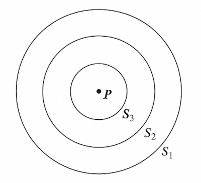
Assuming volume $\Delta V$ and average charge density $\overline{\rho}_{\Delta V}$, we have:

$$ \iint_S \mathbf{E} \cdot \hat{\mathbf{n}} \, dS = \frac{\overline{\rho}_{\Delta V} \Delta V}{\epsilon_0} \tag{II-15} $$

As expected, both sides go to zero as $\Delta V \to 0$. To isolate the quantity that does not go to zero, we divide both sides by $\Delta V$:

$$ \frac{1}{\Delta V} \iint_S \mathbf{E} \cdot \hat{\mathbf{n}} \, dS = \frac{\overline{\rho}_{\Delta V}}{\epsilon_0} $$

Taking the limit as $\Delta V \to 0$, we get:

$$ \lim_{\substack{\Delta V \to 0 \\[0.3em] \text{about}\; (x,y,z)}} \frac{1}{\Delta V} \iint_S \mathbf{E} \cdot \hat{\mathbf{n}} \, dS = \frac{\rho(x, y, z)}{\epsilon_0} \tag{II-16} $$

The Divergence

We define the divergence of a vector field $\mathbf{F}$ as:

$$ \text{div} \, \mathbf{F} \equiv \lim_{\substack{\Delta V \to 0 \\[0.3em] \text{about}\; (x,y,z)}} \frac{1}{\Delta V} \iint_S \mathbf{F} \cdot \hat{\mathbf{n}} \, dS \tag{II-17} $$

Then equation (II-16) can be written as:

$$ \text{div} \, \mathbf{E} = \frac{\rho}{\epsilon_0} \tag{II-18} $$

To calculate this, consider a small cube centered at $(x, y, z)$ with side length $\Delta x$, $\Delta y$, and $\Delta z$:

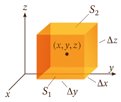
$S_1$ is the front face, $S_2$ is the back face. Let $\mathbf{F} \cdot \mathbf{i} = F_x$.

Then the surface integral over $S_1$ is:

$$ \iint_{S_1} F_x(x, y, z) \, dS \approx F_x(x + \frac{\Delta x}{2}, y, z) \Delta y \Delta z \tag{II-19} $$

Similarly, the surface integral over $S_2$ is:

$$ \iint_{S_2} F_x(x, y, z) \, dS \approx -F_x(x - \frac{\Delta x}{2}, y, z) \Delta y \Delta z \tag{II-20} $$

Then, adding these two and dividing by $\Delta V$ gives:

$$ \frac{1}{\Delta V} \iint_{S_1 + S_2} \mathbf{F} \cdot \hat{\mathbf{n}} \, dS \approx \frac{F_x(x + \frac{\Delta x}{2}, y, z) - F_x(x - \frac{\Delta x}{2}, y, z)}{\Delta x} \tag{II-21} $$

Taking the limit as $\Delta V \to 0$, we get:

$$ \lim_{\Delta V \to 0} \frac{1}{\Delta V} \iint_{S_1 + S_2} \mathbf{F} \cdot \hat{\mathbf{n}} \, dS = \dfrac{\partial F_x}{\partial x} $$

Similarly, we can calculate the contributions from the other two pairs of faces. Then adding all together, we have:

$$ \text{div} \, \mathbf{F} = \dfrac{\partial F_x}{\partial x} + \dfrac{\partial F_y}{\partial y} + \dfrac{\partial F_z}{\partial z} \tag{II-22} $$

It can be shown that the result is independent of the shape of the volume we used.

Differential Form of Gauss’s Law

Combining equations (II-18) and (II-22), we get the differential form of Gauss’s Law:

$$ \frac{\partial E_x}{\partial x} + \frac{\partial E_y}{\partial y} + \frac{\partial E_z}{\partial z} = \frac{\rho}{\epsilon_0} \tag{II-23} $$

The Divergence in Cylindrical Coordinates

Equation (II-22) is merely the divergence in Cartesian coordinates. We prefer to define the divergence as the limit of flux to volume as stated in equation (II-16).

To calculate the divergence in cylindrical coordinates, consider the “cylindrical cuboid” shown below:

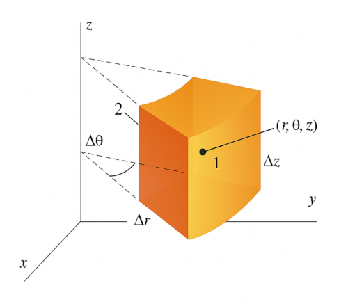
Center is $(r, \theta, z)$, and volume is $\Delta V = r \Delta r \Delta \theta \Delta z$.

The flux of $\mathbf{F}$ through face 1 is:

$$ \iint_{S_1} \mathbf{F} \cdot \hat{\mathbf{n}} \, dS \approx F_r\left(r + \frac{\Delta r}{2}, \theta, z\right) \left(r + \frac{\Delta r}{2}\right) \Delta \theta \Delta z $$

While the flux through face 2 is:

$$ \iint_{S_2} \mathbf{F} \cdot \hat{\mathbf{n}} \, dS \approx -F_r\left(r - \frac{\Delta r}{2}, \theta, z\right) \left(r - \frac{\Delta r}{2}\right) \Delta \theta \Delta z $$

Adding these two and dividing by $\Delta V$ gives, and taking the limit as $\Delta V \to 0$ we get:

$$ \frac{1}{r} \frac{\partial}{\partial r} \left(r F_r\right) $$

Arguing similarly for the other two pairs of faces, we get:

$$ \text{div} \, \mathbf{F} = \frac{1}{r} \frac{\partial}{\partial r} \left(r F_r\right) + \frac{1}{r} \frac{\partial F_\theta}{\partial \theta} + \frac{\partial F_z}{\partial z} \tag{II-24} $$

The Del Notation

We define the del operator as:

$$ \nabla = \mathbf{i} \frac{\partial}{\partial x} + \mathbf{j} \frac{\partial}{\partial y} + \mathbf{k} \frac{\partial}{\partial z} $$

Then, the divergence can be written as:

$$ \text{div} \, \mathbf{F} = \nabla \cdot \mathbf{F} = \frac{\rho}{\epsilon_0} $$

The Divergence Theorem

The divergence theorem states that the flux of a vector field $\mathbf{F}$ through a closed surface $S$ is equal to the integral of the divergence of $\mathbf{F}$ over the volume $V$ enclosed by $S$:

$$ \iint_S \mathbf{F} \cdot \hat{\mathbf{n}} \, dS = \iiint_V \nabla \cdot \mathbf{F} \, dV \tag{II-30} $$

An Example

Divergence theorem on the upper unit hemisphere. Let

$$ \mathbf F(x,y,z)=\mathbf{i}x+\mathbf{j}y+\mathbf{k}z , \quad V=\left\{(x,y,z)\;\middle|\;x^{2}+y^{2}+z^{2}\le 1,\;z\ge 0\right\}. $$

The boundary $S$ has two pieces

• $S_1$ – the curved spherical cap ($x^{2}+y^{2}+z^{2}=1,\\;z\ge 0$),
• $S_2$ – the flat unit disk ($z=0,\\;x^{2}+y^{2}\le 1$).

1 . Volume integral of the divergence

$$ \nabla\!\cdot\!\mathbf F = \frac{\partial x}{\partial x} + \frac{\partial y}{\partial y} + \frac{\partial z}{\partial z} = 1+1+1 = 3. $$

Volume of the hemisphere: $\displaystyle \dfrac12\\!\left(\dfrac{4\pi}{3}\right)=\dfrac{2\pi}{3}$.

$$ \iiint_{V} (\nabla\!\cdot\!\mathbf F)\,dV =3\left(\dfrac{2\pi}{3}\right) =2\pi $$

2 . Flux through the boundary

Curved cap $S_1$

On the unit sphere the outward unit normal is $\hat{\mathbf{n}}=\mathbf{i}x + \mathbf{j}y + \mathbf{k}z$. So, $\mathbf F\\!\cdot\\!\hat{\mathbf{n}} = x^{2}+y^{2}+z^{2}=1.$

$$ \iint_{S_1}\mathbf F\!\cdot\!\hat{\mathbf{n}}\,dS = 1\cdot 2\pi = 2\pi $$

Flat disk $S_2$

Outward normal is $\hat{\mathbf{n}}=-\mathbf k$. On $S_2$, $z=0$. So, $\mathbf F\\!\cdot\\!\hat{\mathbf{n}} = 0$.

$$ \iint_{S_2}\mathbf F\!\cdot\!\hat{\mathbf{n}}\,dS = 0 $$

Total outward flux

$$ \iint_{S}\mathbf F\!\cdot\!\hat{\mathbf{n}}\,dS =2\pi + 0 = 2 \pi $$

Therefore, we have:

$$ \iiint_{V} (\nabla\!\cdot\!\mathbf F)\,dV \;=\; \iint_{S}\mathbf F\!\cdot\!\hat{\mathbf{n}}\,dS \;=\;2\pi $$

Applications

We want to derive equation (II-18):

$$ \text{div} \, \mathbf{E} = \frac{\rho}{\epsilon_0} $$

We start with Gauss’s Law:

$$ \iint_S \mathbf{E} \cdot \hat{\mathbf{n}} \, dS = \frac{1}{\epsilon_0} \iiint_V \rho \, dV \tag{II-31} $$

We can use the divergence theorem to rewrite the left-hand side:

$$ \iint_S \mathbf{E} \cdot \hat{\mathbf{n}} \, dS = \iiint_V \nabla \cdot \mathbf{E} \, dV \tag{II-32} $$

Combining equations (II-31) and (II-32), we get:

$$ \iiint_V \nabla \cdot \mathbf{E} \, dV = \frac{1}{\epsilon_0} \iiint_V \rho \, dV $$

Since this is true for any volume $V$, we can conclude that:

$$ \nabla \cdot \mathbf{E} = \frac{\rho}{\epsilon_0} $$